import pandas as pd
import numpy as np
from sklearn.linear_model import LinearRegression
from sklearn.model_selection import train_test_split, KFold, cross_val_score
from sklearn import metrics
import statsmodels.formula.api as smf

# visualization
import seaborn as sns
import matplotlib.pyplot as plt
%matplotlib inline2 Linear Regression
3 Part 1: Introduction
- Classification problem: supervised learning problem with a categorical response
- Regression problem: supervised learning problem with a continuous response
- Linear regression: machine learning model that can be used for regression problems
Why are we learning linear regression?
- widely used
- runs fast
- easy to use (no tuning is required)
- highly interpretable
- basis for many other methods
Lesson goals:
- Conceptual understanding of linear regression and how it “works”
- Familiarity with key terminology
- Ability to apply linear regression to a machine learning problem using scikit-learn
- Ability to interpret model coefficients
- Familiarity with different approaches for feature selection
- Understanding of three different evaluation metrics for regression
- Understanding of linear regression’s strengths and weaknesses
3.1 Libraries
- Statsmodels: “statistics in Python”
- robust functionality for linear modeling
- useful for teaching purposes
- will not be used in the course outside of this lesson
- scikit-learn: “machine learning in Python”
- significantly more functionality for general purpose machine learning
3.2 Reading the advertising data
# read data into a DataFrame
data = pd.read_csv('https://raw.githubusercontent.com/marcopeix/ISL-linear-regression/refs/heads/master/data/Advertising.csv', index_col=0)
data.head()| TV | radio | newspaper | sales | |
|---|---|---|---|---|
| 1 | 230.1 | 37.8 | 69.2 | 22.1 |
| 2 | 44.5 | 39.3 | 45.1 | 10.4 |
| 3 | 17.2 | 45.9 | 69.3 | 9.3 |
| 4 | 151.5 | 41.3 | 58.5 | 18.5 |
| 5 | 180.8 | 10.8 | 58.4 | 12.9 |
What are the observations?
- Each observation represents one market (200 markets in the dataset)
What are the features?
- TV: advertising dollars spent on TV for a single product (in thousands of dollars)
- Radio: advertising dollars spent on Radio
- Newspaper: advertising dollars spent on Newspaper
What is the response?
- Sales: sales of a single product in a given market (in thousands of widgets)
3.3 Questions about the data
You are asked by the company: On the basis of this data, how should we spend our advertising money in the future?
You come up with more specific questions:
- Is there a relationship between ads and sales?
- How strong is that relationship?
- Which ad types contribute to sales?
- What is the effect of each ad type of sales?
- Given ad spending in a particular market, can sales be predicted?
3.4 Visualizing the data
Use a scatter plot to visualize the relationship between the features and the response.
# scatter plot in Seaborn
sns.pairplot(data, x_vars=['TV','radio','newspaper'], y_vars='sales', size=6, aspect=0.7)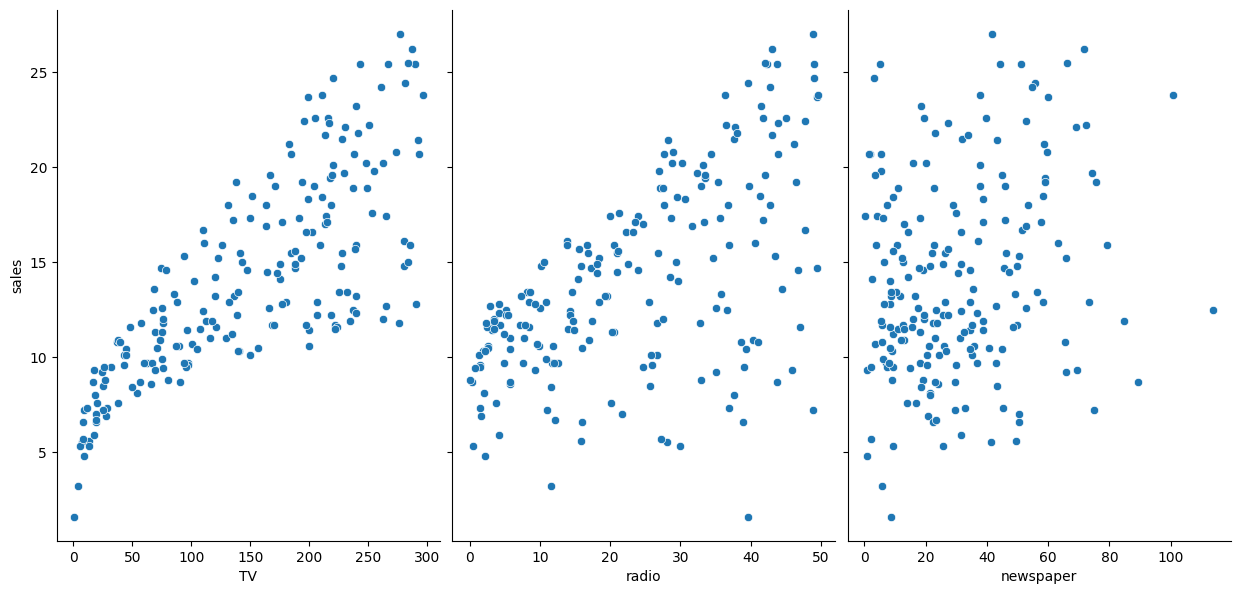
# include a "regression line"
sns.pairplot(data, x_vars=['TV','radio','newspaper'], y_vars='sales', size=6, aspect=0.7, kind='reg')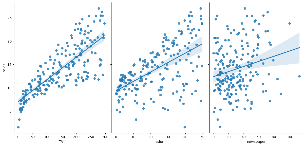
# scatter plot in Pandas
fig, axs = plt.subplots(1, 3, sharey=True)
data.plot(kind='scatter', x='TV', y='sales', ax=axs[0], figsize=(16, 6))
data.plot(kind='scatter', x='radio', y='sales', ax=axs[1])
data.plot(kind='scatter', x='newspaper', y='sales', ax=axs[2])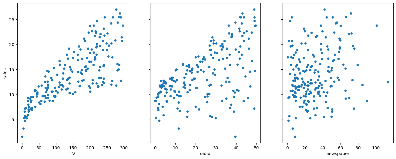
Use a scatter matrix to visualize the relationship between all numerical variables.
# scatter matrix in Seaborn
sns.pairplot(data)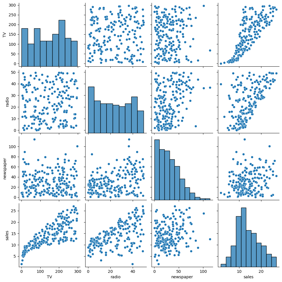
# scatter matrix in Pandas
pd.plotting.scatter_matrix(data, figsize=(12, 10))
array([[<Axes: xlabel='TV', ylabel='TV'>,
<Axes: xlabel='radio', ylabel='TV'>,
<Axes: xlabel='newspaper', ylabel='TV'>,
<Axes: xlabel='sales', ylabel='TV'>],
[<Axes: xlabel='TV', ylabel='radio'>,
<Axes: xlabel='radio', ylabel='radio'>,
<Axes: xlabel='newspaper', ylabel='radio'>,
<Axes: xlabel='sales', ylabel='radio'>],
[<Axes: xlabel='TV', ylabel='newspaper'>,
<Axes: xlabel='radio', ylabel='newspaper'>,
<Axes: xlabel='newspaper', ylabel='newspaper'>,
<Axes: xlabel='sales', ylabel='newspaper'>],
[<Axes: xlabel='TV', ylabel='sales'>,
<Axes: xlabel='radio', ylabel='sales'>,
<Axes: xlabel='newspaper', ylabel='sales'>,
<Axes: xlabel='sales', ylabel='sales'>]], dtype=object)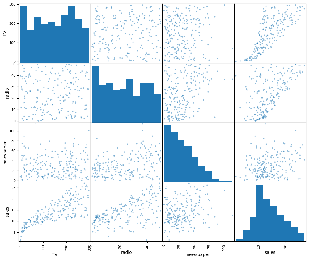
Use a correlation matrix to visualize the correlation between all numerical variables.
# compute correlation matrix
data.corr()| TV | radio | newspaper | sales | |
|---|---|---|---|---|
| TV | 1.000000 | 0.054809 | 0.056648 | 0.782224 |
| radio | 0.054809 | 1.000000 | 0.354104 | 0.576223 |
| newspaper | 0.056648 | 0.354104 | 1.000000 | 0.228299 |
| sales | 0.782224 | 0.576223 | 0.228299 | 1.000000 |
# display correlation matrix in Seaborn using a heatmap
sns.heatmap(data.corr())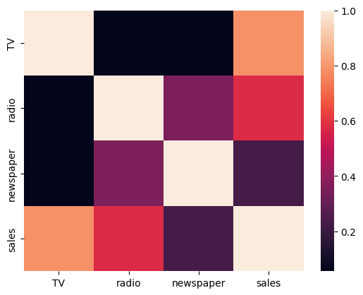
Correlation is a quantification of how two variables are related in a linear fashion
But does NOT reveal if there is any causation between variables
In general, machine learning is great at revealing when variables are correlated, but not if there is any causation between them
4 Part 2: Simple linear regression
Simple linear regression is an approach for predicting a continuous response using a single feature. It takes the following form:
\(y = \beta_0 + \beta_1x\)
- \(y\) is the response
- \(x\) is the feature
- \(\beta_0\) is the intercept
- \(\beta_1\) is the coefficient for x
\(\beta_0\) and \(\beta_1\) are called the model coefficients:
- We must “learn” the values of these coefficients to create our model.
- And once we’ve learned these coefficients, we can use the model to predict Sales.
4.1 Estimating (“learning”) model coefficients
- Coefficients are estimated during the model fitting process using the least squares criterion.
- We are find the line (mathematically) which minimizes the sum of squared residuals (or “sum of squared errors”).
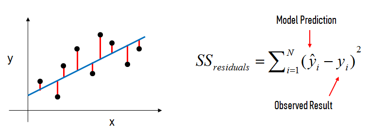
In this diagram:
- The black dots are the observed values of x and y.
- The blue line is our least squares line.
- The red lines are the residuals, which are the distances between the observed values and the least squares line.
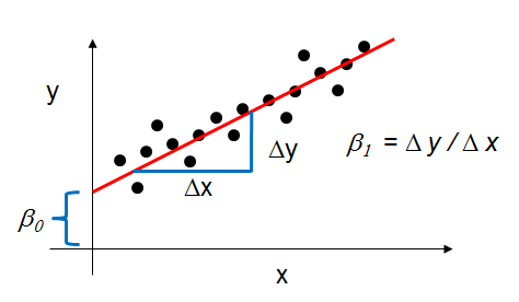
How do the model coefficients relate to the least squares line?
- \(\beta_0\) is the intercept (the value of \(y\) when \(x\)=0)
- \(\beta_1\) is the slope (the change in \(y\) divided by change in \(x\))
Let’s estimate the model coefficients for the advertising data:
### STATSMODELS ###

# create a fitted model
lm = smf.ols(formula='sales ~ TV', data=data).fit()

# print the coefficients
lm.params
Intercept 7.032594
TV 0.047537
dtype: float64### SCIKIT-LEARN ###
# create X and y
feature_cols = ['TV']
X = data[feature_cols]
y = data.sales
# instantiate and fit
linreg = LinearRegression()
linreg.fit(X, y)
# print the coefficients
print(linreg.intercept_)
print(linreg.coef_)7.032593549127695
[0.04753664]4.2 Interpreting model coefficients
How do we interpret the TV coefficient (\(\beta_1\))?
- A “unit” increase in TV ad spending is associated with a 0.0475 “unit” increase in Sales.
- Meaning: An additional $1,000 spent on TV ads is associated with an increase in sales of 47.5 widgets.
- This is not a statement of causation.
If an increase in TV ad spending was associated with a decrease in sales, \(\beta_1\) would be negative.
4.3 Using the model for prediction
Let’s say that there was a new market where the TV advertising spend was $50,000. What would we predict for the Sales in that market?
\[y = \beta_0 + \beta_1x\] \[y = 7.0326 + 0.0475 \times 50\]
# manually calculate the prediction
7.0326 + 0.0475*509.4076### STATSMODELS ###
# you have to create a DataFrame since the Statsmodels formula interface expects it
X_new = pd.DataFrame({'TV': [50]})
# predict for a new observation
lm.predict(X_new)0 9.409426
dtype: float64### SCIKIT-LEARN ###
# predict for a new observation
linreg.predict([[50]])array([9.40942557])Thus, we would predict Sales of 9,409 widgets in that market.
4.4 Does the scale of the features matter?
Let’s say that TV was measured in dollars, rather than thousands of dollars. How would that affect the model?
data['TV_dollars'] = data.TV * 1000
data.head()| TV | radio | newspaper | sales | TV_dollars | |
|---|---|---|---|---|---|
| 1 | 230.1 | 37.8 | 69.2 | 22.1 | 230100.0 |
| 2 | 44.5 | 39.3 | 45.1 | 10.4 | 44500.0 |
| 3 | 17.2 | 45.9 | 69.3 | 9.3 | 17200.0 |
| 4 | 151.5 | 41.3 | 58.5 | 18.5 | 151500.0 |
| 5 | 180.8 | 10.8 | 58.4 | 12.9 | 180800.0 |
### SCIKIT-LEARN ###

# create X and y
feature_cols = ['TV_dollars']
X = data[feature_cols]
y = data.sales

# instantiate and fit
linreg = LinearRegression()
linreg.fit(X, y)

# print the coefficients
print(linreg.intercept_)
print(linreg.coef_)
7.032593549127694
[4.75366404e-05]How do we interpret the TV_dollars coefficient (\(\beta_1\))?
- A “unit” increase in TV ad spending is associated with a 0.0000475 “unit” increase in Sales.
- Meaning: An additional dollar spent on TV ads is associated with an increase in sales of 0.0475 widgets.
- Meaning: An additional $1,000 spent on TV ads is associated with an increase in sales of 47.5 widgets.
# predict for a new observation
linreg.predict(50000)
array([ 9.40942557])The scale of the features is irrelevant for linear regression models, since it will only affect the scale of the coefficients, and we simply change our interpretation of the coefficients.
5 Part 3: A deeper understanding
5.1 Bias and variance
Linear regression is a low variance/high bias model:
- Low variance: Under repeated sampling from the underlying population, the line will stay roughly in the same place
- High bias: The line will rarely fit the data well
A closely related concept is confidence intervals.
5.2 Confidence intervals
Statsmodels calculates 95% confidence intervals for our model coefficients, which are interpreted as follows: If the population from which this sample was drawn was sampled 100 times, approximately 95 of those confidence intervals would contain the “true” coefficient.
### STATSMODELS ###

# print the confidence intervals for the model coefficients
lm.conf_int()| 0 | 1 | |
|---|---|---|
| Intercept | 6.129719 | 7.935468 |
| TV | 0.042231 | 0.052843 |
- We only have a single sample of data, and not the entire population of data.
- The “true” coefficient is either within this interval or it isn’t, but there’s no way to actually know.
- We estimate the coefficient with the data we do have, and we show uncertainty about that estimate by giving a range that the coefficient is probably within.
- From Quora: What is a confidence interval in layman’s terms?
Note: 95% confidence intervals are just a convention. You can create 90% confidence intervals (which will be more narrow), 99% confidence intervals (which will be wider), or whatever intervals you like.
A closely related concept is hypothesis testing.
5.3 Hypothesis testing and p-values
General process for hypothesis testing:
- You start with a null hypothesis and an alternative hypothesis (that is opposite the null).
- You check whether the data supports rejecting the null hypothesis or failing to reject the null hypothesis.
For model coefficients, here is the conventional hypothesis test:
- null hypothesis: There is no relationship between TV ads and Sales (and thus \(\beta_1\) equals zero)
- alternative hypothesis: There is a relationship between TV ads and Sales (and thus \(\beta_1\) is not equal to zero)
How do we test this hypothesis?
- The p-value is the probability that the relationship we are observing is occurring purely by chance.
- If the 95% confidence interval for a coefficient does not include zero, the p-value will be less than 0.05, and we will reject the null (and thus believe the alternative).
- If the 95% confidence interval includes zero, the p-value will be greater than 0.05, and we will fail to reject the null.
### STATSMODELS ###

# print the p-values for the model coefficients
lm.pvalues
Intercept 1.406300e-35
TV 1.467390e-42
dtype: float64Thus, a p-value less than 0.05 is one way to decide whether there is likely a relationship between the feature and the response. In this case, the p-value for TV is far less than 0.05, and so we believe that there is a relationship between TV ads and Sales.
Note that we generally ignore the p-value for the intercept.
5.4 How well does the model fit the data?
R-squared:
- A common way to evaluate the overall fit of a linear model
- Defined as the proportion of variance explained, meaning the proportion of variance in the observed data that is explained by the model
- Also defined as the reduction in error over the null model, which is the model that simply predicts the mean of the observed response
- Between 0 and 1, and higher is better
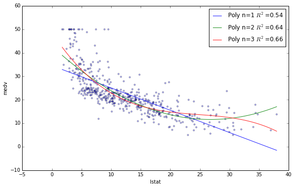
Here’s an example of what R-squared “looks like”:
Let’s calculate the R-squared value for our simple linear model:
### STATSMODELS ###

# print the R-squared value for the model
print(lm.rsquared)0.611875050850071### SCIKIT-LEARN ###
# calculate the R-squared value for the model
y_pred = linreg.predict(X)
metrics.r2_score(y, y_pred)0.611875050850071- The threshold for a “good” R-squared value is highly dependent on the particular domain.
- R-squared is more useful as a tool for comparing models.
6 Part 4: Multiple Linear Regression
Simple linear regression can easily be extended to include multiple features, which is called multiple linear regression:
\(y = \beta_0 + \beta_1x_1 + ... + \beta_nx_n\)
Each \(x\) represents a different feature, and each feature has its own coefficient:
\(y = \beta_0 + \beta_1 \times TV + \beta_2 \times Radio + \beta_3 \times Newspaper\)
### SCIKIT-LEARN ###

# create X and y
feature_cols = ['TV', 'radio', 'newspaper']
X = data[feature_cols]
y = data.sales

# instantiate and fit
linreg = LinearRegression()
linreg.fit(X, y)

# print the coefficients
print(linreg.intercept_)
print(linreg.coef_)
2.938889369459412
[ 0.04576465 0.18853002 -0.00103749]# pair the feature names with the coefficients
zip(feature_cols, linreg.coef_)[('TV', 0.045764645455397601),
('Radio', 0.18853001691820456),
('Newspaper', -0.0010374930424762725)]For a given amount of Radio and Newspaper spending, an increase of $1000 in TV spending is associated with an increase in Sales of 45.8 widgets.
For a given amount of TV and Newspaper spending, an increase of $1000 in Radio spending is associated with an increase in Sales of 188.5 widgets.
For a given amount of TV and Radio spending, an increase of $1000 in Newspaper spending is associated with an decrease in Sales of 1.0 widgets. How could that be?
6.1 Feature selection
How do I decide which features to include in a linear model?
6.1.1 Using p-values
We could try a model with all features, and only keep features in the model if they have small p-values:
### STATSMODELS ###

# create a fitted model with all three features
lm = smf.ols(formula='sales ~ TV + radio + newspaper', data=data).fit()

# print the p-values for the model coefficients
print(lm.pvalues)
Intercept 1.267295e-17
TV 1.509960e-81
radio 1.505339e-54
newspaper 8.599151e-01
dtype: float64This indicates we would reject the null hypothesis for TV and Radio (that there is no association between those features and Sales), and fail to reject the null hypothesis for Newspaper. Thus, we would keep TV and Radio in the model.
However, this approach has drawbacks:
- Linear models rely upon a lot of assumptions (such as the features being independent), and if those assumptions are violated (which they usually are), p-values are less reliable.
- Using a p-value cutoff of 0.05 means that if you add 100 features to a model that are pure noise, 5 of them (on average) will still be counted as significant.
6.1.2 Using R-squared
We could try models with different sets of features, and compare their R-squared values:
# R-squared value for the model with two features
lm = smf.ols(formula='sales ~ TV + radio', data=data).fit()
print(lm.rsquared)0.8971942610828956# R-squared value for the model with three features
lm = smf.ols(formula='sales ~ TV + radio + newspaper', data=data).fit()
print(lm.rsquared)0.8972106381789522This would seem to indicate that the best model includes all three features. Is that right?
- R-squared will always increase as you add more features to the model, even if they are unrelated to the response.
- As such, using R-squared as a model evaluation metric can lead to overfitting.
- Adjusted R-squared is an alternative that penalizes model complexity (to control for overfitting), but it generally under-penalizes complexity.
As well, R-squared depends on the same assumptions as p-values, and it’s less reliable if those assumptions are violated.
6.1.3 Using train/test split (or cross-validation)
A better approach to feature selection!
- They attempt to directly estimate how well your model will generalize to out-of-sample data.
- They rely on fewer assumptions that linear regression.
- They can easily be applied to any model, not just linear models.
6.2 Evaluation metrics for regression problems
Evaluation metrics for classification problems, such as accuracy, are not useful for regression problems. We need evaluation metrics designed for comparing continuous values.
Let’s create some example numeric predictions, and calculate three common evaluation metrics for regression problems:
# define true and predicted response values
y_true = [100, 50, 30, 20]
y_pred = [90, 50, 50, 30]
Mean Absolute Error (MAE) is the mean of the absolute value of the errors:
\[\frac 1n\sum_{i=1}^n|y_i-\hat{y}_i|\]
print(metrics.mean_absolute_error(y_true, y_pred))10.0Mean Squared Error (MSE) is the mean of the squared errors:
\[\frac 1n\sum_{i=1}^n(y_i-\hat{y}_i)^2\]
print(metrics.mean_squared_error(y_true, y_pred))150.0Root Mean Squared Error (RMSE) is the square root of the mean of the squared errors:
\[\sqrt{\frac 1n\sum_{i=1}^n(y_i-\hat{y}_i)^2}\]
print(np.sqrt(metrics.mean_squared_error(y_true, y_pred)))12.24744871391589Comparing these metrics:
- MAE is the easiest to understand, because it’s the average error.
- MSE is more popular than MAE, because MSE “punishes” larger errors, which tends to be useful in the real world.
- RMSE is even more popular than MSE, because RMSE is interpretable in the “y” units.
All of these are loss functions, because we want to minimize them.
Here’s an additional example, to demonstrate how MSE/RMSE punish larger errors:
# same true values as above
y_true = [100, 50, 30, 20]

# new set of predicted values
y_pred = [60, 50, 30, 20]

# MAE is the same as before
print(metrics.mean_absolute_error(y_true, y_pred))

# RMSE is larger than before
print(np.sqrt(metrics.mean_squared_error(y_true, y_pred)))
10.0
20.06.3 Using train/test split for feature selection
Let’s use train/test split with RMSE to decide whether Newspaper should be kept in the model:
# define a function that accepts X and y and computes testing RMSE
def train_test_rmse(X, y):
    X_train, X_test, y_train, y_test = train_test_split(X, y, random_state=1)
    linreg = LinearRegression()
    linreg.fit(X_train, y_train)
    y_pred = linreg.predict(X_test)
    return np.sqrt(metrics.mean_squared_error(y_test, y_pred))
# include Newspaper
feature_cols = ['TV', 'radio', 'newspaper']
X = data[feature_cols]
train_test_rmse(X, y)np.float64(1.404651423032896)# exclude Newspaper
feature_cols = ['TV', 'radio']
X = data[feature_cols]
print(train_test_rmse(X, y))1.38790346993828886.4 Comparing linear regression with other models
Advantages of linear regression:
- Simple to explain
- Highly interpretable
- Model training and prediction are fast
- No tuning is required (excluding regularization)
- Features don’t need scaling
- Can perform well with a small number of observations
Disadvantages of linear regression:
- Presumes a linear relationship between the features and the response
- Performance is (generally) not competitive with the best supervised learning methods due to high bias
- Sensitive to irrelevant features
- Can’t automatically learn feature interactions
6.4.1 Referensi
https://github.com/sinanuozdemir